Visualizing and Maintaining the Green Canopy of NYC
Author
Chhin Lama
Introduction
New York City’s extensive network of more than 650,000 street trees plays a critical role in cooling neighborhoods, improving air quality, and enhancing everyday quality of life. This project analyzes the NYC Street Tree Census and council district boundaries to understand the spatial distribution, species composition, and health of the city’s urban canopy. Through mapping and district-level analytics, we identify areas with strong coverage and others that require targeted planting or maintenance to advance canopy equity across the city.
Note
Outline of This Report
In Task 1, we download and process the NYC City Council District boundaries using spatial data from the Department of City Planning.
In Task 2, we retrieve and combine NYC Tree Points data from the OpenData API using responsible pagination and caching.
In Task 3, we map all tree locations across council districts using ggplot2 and sf, visualizing the city’s green canopy.
In Task 4, we conduct district-level analyses to identify areas with the most trees, highest density, and greatest need for maintenance.
Finally, In Task 5, we design a Parks Department Proposal recommending targeted investments to enhance canopy equity and urban sustainability.
Data Acquisition
NYC CITY COUNCIL DISTRICTS
Task 1: Download NYC City Council District Boundaries
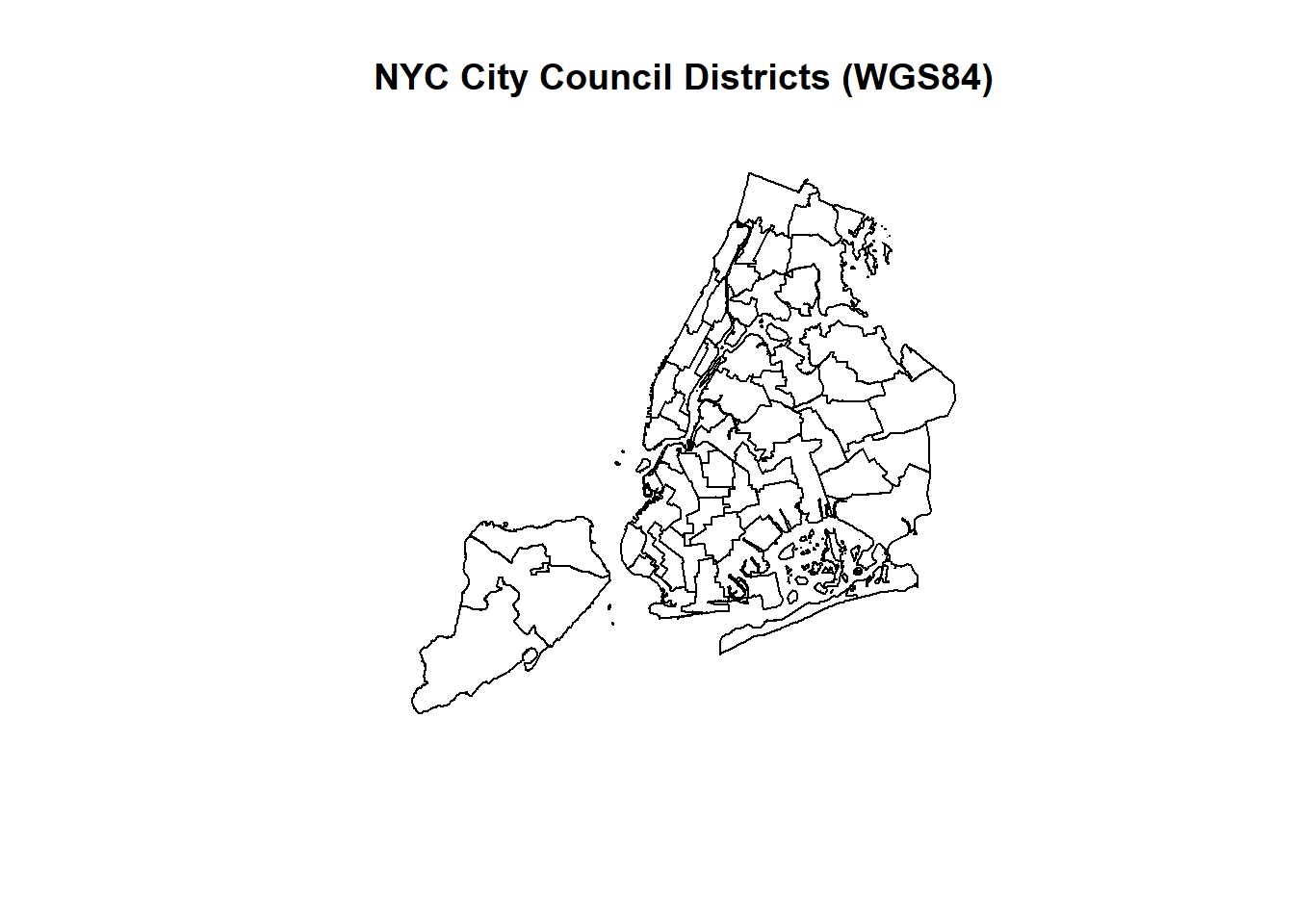
The first step involves acquiring the official shapefile of New York City’s 51 Council Districts from the NYC Department of City Planning to establish a geographic framework for analysis. This dataset provides the spatial boundaries necessary to align tree locations with their respective council districts, enabling district-level comparisons and analyses throughout the project.
Code
# Install (only if needed)pkgs <-c("sf", "dplyr", "readr", "httr2", "withr")new_pkgs <- pkgs[!pkgs %in%installed.packages()[, "Package"]]if (length(new_pkgs)) install.packages(new_pkgs)# Loadlibrary(sf)library(dplyr)library(readr)library(httr2)library(withr)# .zip link from DCP:council_zip_url <-"nycc_25c.zip"unzip("data/mp03/nycc_25c.zip", exdir ="data/mp03/nycc_25c")# --- Locate the .shp inside the unzipped folder (recursive in case DCP nested subfolders) ---shp_file <-list.files("data/mp03/nycc_25c",pattern ="\\.shp$", full.names =TRUE, recursive =TRUE)if (length(shp_file) ==0) {stop("No .shp found under data/mp03/nycc_25c. Re-check unzip. Try: unzip('data/mp03/nycc_25c.zip', list = TRUE)")}# --- Read, transform, (optionally) simplify ---districts <- sf::st_read(shp_file[1], quiet =TRUE)districts <- sf::st_transform(districts, crs ="WGS84")# Optional: simplify for faster plotting (tweak tolerance if edges look too coarse)districts <- districts %>%mutate(geometry = sf::st_simplify(geometry, dTolerance =5))# --- Quick plot ---plot(sf::st_geometry(districts), main ="NYC City Council Districts (WGS84)")
Code
get_nyc_council_districts <-function( zip_url_or_path, # either HTTPS URL from DCP OR a local path like "data/mp03/nycc_25c.zip"data_dir ="data/mp03", # where to store zip/unzipzip_name =NULL, # optional; defaults to basename(zip_url_or_path)unzip_dir_name ="nycc_25c", # folder to unzip intosimplify_tol_m =NA# e.g., 5 (meters) for faster plotting; NA to skip) {# 1) Ensure data dir existsdir.create(data_dir, recursive =TRUE, showWarnings =FALSE)# 2) Resolve zip path (download only if needed)if (is.null(zip_name)) zip_name <-basename(zip_url_or_path) zip_path <-file.path(data_dir, zip_name) unzip_dir <-file.path(data_dir, unzip_dir_name) is_url <-grepl("^https?://", zip_url_or_path, ignore.case =TRUE)if (!file.exists(zip_path)) {if (is_url) {message("Downloading zip once to: ", zip_path)download.file(zip_url_or_path, destfile = zip_path, mode ="wb", quiet =FALSE) } else {# treat input as local file the user already has (e.g., "data/mp03/nycc_25c.zip")if (!file.exists(zip_url_or_path)) {stop("Local zip not found: ", zip_url_or_path) }file.copy(zip_url_or_path, zip_path, overwrite =FALSE)message("Copied local zip to project data dir: ", zip_path) } } else {message("Zip already present: ", zip_path) }# 3) Unzip only if neededif (!dir.exists(unzip_dir)) {message("Unzipping to: ", unzip_dir)unzip(zip_path, exdir = unzip_dir) } else {message("Already unzipped: ", unzip_dir) }# 4) Find .shp inside unzipped dir (recursive in case DCP nested folders) shp_files <-list.files(unzip_dir, pattern ="\\.shp$", full.names =TRUE, recursive =TRUE)if (length(shp_files) ==0) {# Helpful debugging hintcat("\nNo .shp found. Zip contents:\n")print(unzip(zip_path, list =TRUE))stop("No .shp file found under: ", unzip_dir) }if (length(shp_files) >1) {message("Multiple .shp files found; using the first: ", basename(shp_files[1])) }# 5) Read shapefile districts <- sf::st_read(shp_files[1], quiet =TRUE)# 6) Transform to WGS84 districts <- sf::st_transform(districts, crs ="WGS84")# 7) Optional: simplify for faster plottingif (!is.na(simplify_tol_m)) { districts <- districts %>%mutate(geometry = sf::st_simplify(geometry, dTolerance = simplify_tol_m)) }# 8) Return transformed sfreturn(districts)}
NYC TREE POINTS
Task 2: Download Tree Points
To analyze the distribution and characteristics of NYC’s urban trees, the next step involves acquiring the NYC Street Tree Census dataset from NYC OpenData. The data was accessed programmatically through the Socrata SODA2 API in GeoJSON format, obtained by selecting the “API Endpoint” option under the dataset’s export menu. This approach ensures responsible, reproducible data collection directly from the city’s open data portal.
Code
library(sf)library(dplyr)library(purrr)get_nyc_tree_points <-function(base_url ="https://data.cityofnewyork.us/resource/nwxe-4ae8.geojson", # NYC Street Tree Census pointsdata_dir ="data/mp03",file_prefix ="trees",limit =50000, # safe page size (bigger = fewer requests; too big = risk timeouts)start_offset =0,max_pages =Inf, # safety cap; keep Inf to read everythingsleep_sec =0.2, # be polite to serverdev_n_pages =NULL, # e.g., 2 to download only 2 pages for developmentextra_params =list() # optional named list for SoQL filters: list(`$select`="...", `$where`="...")) {# Ensure folderdir.create(data_dir, recursive =TRUE, showWarnings =FALSE)# Helper to build page file names page_file <-function(i) file.path(data_dir, sprintf("%s_%03d.geojson", file_prefix, i))# Loop over pages i <-1 offset <- start_offset downloaded_files <-character(0)repeat { fpath <-page_file(i)# Download only if the page file doesn't existif (!file.exists(fpath)) {message(sprintf("Requesting page %d (limit=%d, offset=%d)...", i, limit, offset)) req <-request(base_url) |>req_url_query(`$limit`= limit, `$offset`= offset)# Add any extra SoQL params (optional)if (length(extra_params)) {for (nm innames(extra_params)) { req <-req_url_query(req, !!nm := extra_params[[nm]]) } }# Perform request and save raw GeoJSON resp <-req_perform(req)writeBin(resp_body_raw(resp), fpath) } else {message(sprintf("Page %d already exists: %s (skipping download)", i, basename(fpath))) } downloaded_files <-c(downloaded_files, fpath)# Read the page to see how many rows we got page_sf <-tryCatch(st_read(fpath, quiet =TRUE),error =function(e) {warning(sprintf("Failed to read %s. Deleting and retrying next render.", fpath))try(unlink(fpath))stop(e) } ) n_rows <-nrow(page_sf)message(sprintf("Read page %d with %d rows.", i, n_rows))# Stop if last page (fewer than limit rows)if (n_rows < limit) {message("Reached final page (rows < limit).")break }# Optional dev mode: limit number of pages to speed iterationif (!is.null(dev_n_pages) && i >= dev_n_pages) {message(sprintf("Dev mode: stopping after %d pages.", dev_n_pages))break }# Safety capif (i >= max_pages) {message(sprintf("Reached max_pages=%d. Stopping.", max_pages))break }# Next page i <- i +1 offset <- offset + limit# Be politeSys.sleep(sleep_sec) }# Read ALL saved pages and combinemessage("Combining all downloaded pages…") pages <-lapply(downloaded_files, function(p) st_read(p, quiet =TRUE)) trees_sf <-bind_rows(pages)# GeoJSON returns WGS84 by standard; ensure CRS is set/consistentif (is.na(st_crs(trees_sf))) { trees_sf <-st_set_crs(trees_sf, 4326) # WGS84 (EPSG:4326) } trees_sf}use_dev <-FALSEif (!exists("use_dev")) use_dev <-FALSEif (isTRUE(use_dev)) {# small, fast subset for testingif (file.exists("data/mp03/trees_dev.rds")) { trees <-readRDS("data/mp03/trees_dev.rds") } else { trees <-get_nyc_tree_points(limit =20000, dev_n_pages =2)dir.create("data/mp03", recursive =TRUE, showWarnings =FALSE)saveRDS(trees, "data/mp03/trees_dev.rds") }} else {# FULL DATA — read all saved GeoJSON pages or download them files <-list.files("data/mp03", pattern ="^trees_\\d{3}\\.geojson$", full.names =TRUE)if (length(files) ==0) { trees <-get_nyc_tree_points(limit =50000, dev_n_pages =NULL) } else { trees <-map(files, \(f) { message("Reading ", basename(f)); st_read(f, quiet =TRUE) }) |>bind_rows()if (is.na(st_crs(trees))) trees <-st_set_crs(trees, 4326) }}
Data Integration and Initial Exploration
Mapping NYC Trees
Task 3: Plot All Tree Points
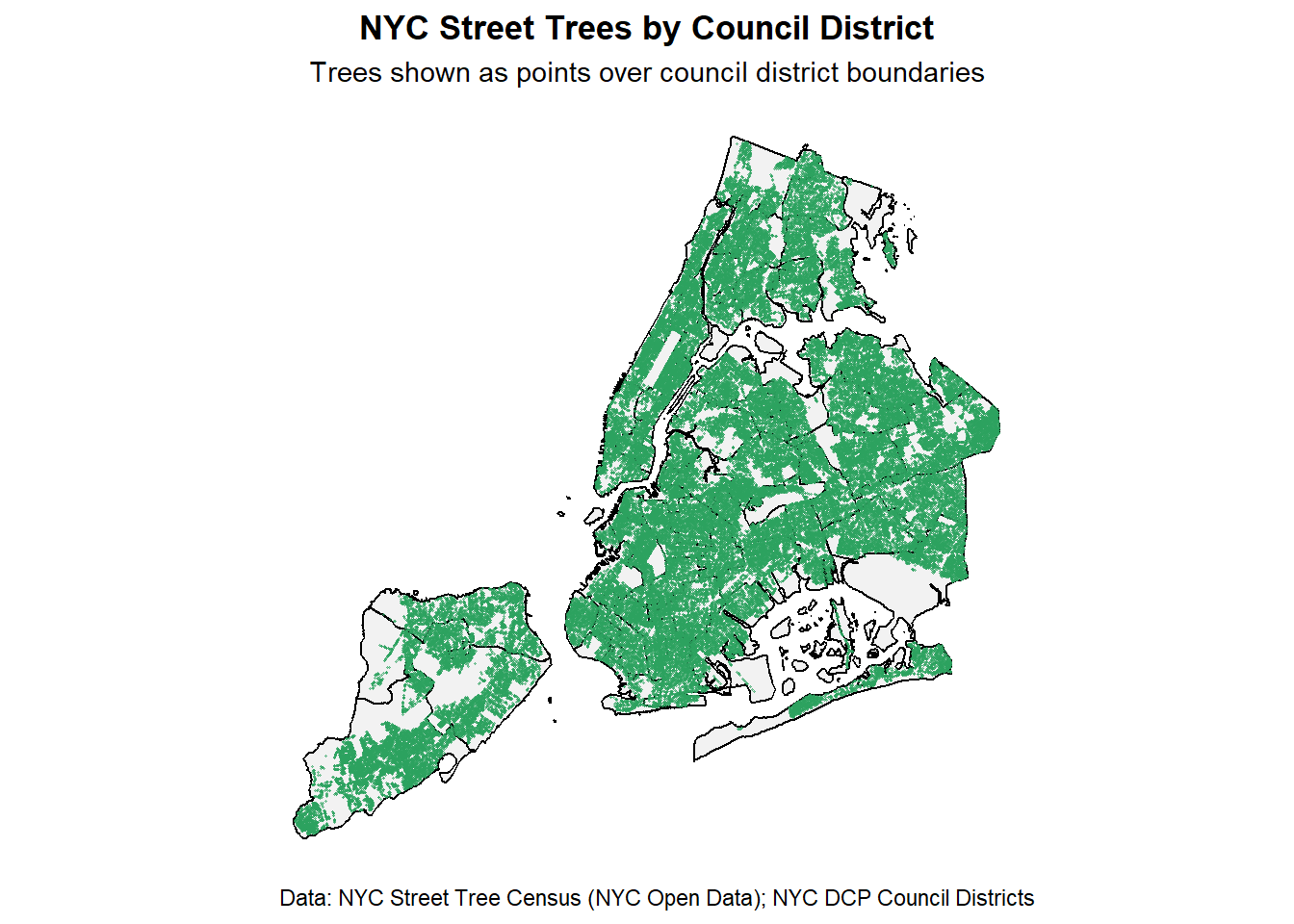
To begin exploring the dataset, it is helpful to visualize the spatial distribution of trees across New York City. By overlaying individual tree locations onto the city’s council district boundaries using ggplot2 and geom_sf(), we can observe overall coverage patterns and identify areas of high or low tree density.
Code
pkgs <-c("ggplot2", "sf", "dplyr")new_pkgs <- pkgs[!pkgs %in%installed.packages()[, "Package"]]if (length(new_pkgs)) install.packages(new_pkgs)library(ggplot2)library(sf)library(dplyr)trees_plot <- treesif (st_crs(trees_plot) !=st_crs(districts)) { trees_plot <-st_transform(trees_plot, st_crs(districts))}set.seed(1)trees_plot_small <- trees_plot |> dplyr::slice_sample(n =min(100000, nrow(trees_plot)))districts_s <- districts |> dplyr::mutate(geometry = sf::st_simplify(geometry, dTolerance =5))ggplot() +geom_sf(data = districts_s,fill ="grey95",color ="black",linewidth =0.4) +geom_sf(data = trees_plot_small,color ="#2ca25f",alpha =0.5,size =0.2) +coord_sf(datum =NA) +theme_minimal(base_size =11) +theme(panel.grid.major =element_line(color ="grey90"),panel.grid.minor =element_blank(),plot.title =element_text(hjust =0.5, face ="bold"),plot.subtitle =element_text(hjust =0.5) ) +labs(title ="NYC Street Trees by Council District",subtitle ="Trees shown as points over council district boundaries",caption ="Data: NYC Street Tree Census (NYC Open Data); NYC DCP Council Districts",x =NULL, y =NULL )
District-Level Analyses of Trees
Task 4: District-Level Analysis of Tree Coverage
We integrate the tree point data with City Council district boundaries using a spatial join to better understand NYC’s urban forest. This allows us to explore several key questions—such as which districts have the most trees, the highest density, or the largest share of dead trees—laying the groundwork for district-level analysis.
Q1. Which council district has the most trees?
Council District 51 has the most trees, with a total of 51,211 - the highest count citywide.
Code
district_counts_attr <- trees |>st_drop_geometry() |>mutate(coun_dist =coalesce(as.integer(council_district), as.integer(cncldist))) |>filter(!is.na(coun_dist)) |>count(coun_dist, name ="total_trees") |>arrange(desc(total_trees))head(district_counts_attr, 10)
caption ="Top 10 NYC Council Districts by Tree Density (trees per km²)"
Q3. Which district has highest fraction of dead trees out of all trees?
District 16 has the highest share of dead trees, with approximately 5.4% of its tree population recorded as dead.
Code
# merge districtsdistrict_base <- districts |>st_drop_geometry() |>rename(coun_dist = CounDist)# get counts of total and dead trees per districtdead_summary <- trees |>st_drop_geometry() |>mutate(coun_dist =coalesce(as.integer(council_district), as.integer(cncldist)) ) |>filter(!is.na(coun_dist)) |>group_by(coun_dist) |>summarise(total_trees =n(),dead_trees =sum(status =="Dead", na.rm =TRUE),frac_dead = dead_trees / total_trees ) |>arrange(desc(frac_dead))head(dead_summary, 10)
Q4. What is the most common tree species in Manhattan?
Honeylocust is the most common species in Manhattan with 13,905 recorded trees.
Code
trees_joined <- trees |>st_drop_geometry() |>mutate(coun_dist =coalesce(as.integer(council_district), as.integer(cncldist)) ) |>filter(!is.na(coun_dist))# Adding new column assigning borough by council district numbertrees_joined <- trees_joined |>mutate(borough =case_when( coun_dist >=1& coun_dist <=10~"Manhattan", coun_dist >=11& coun_dist <=18~"Bronx", coun_dist >=19& coun_dist <=32~"Queens", coun_dist >=33& coun_dist <=48~"Brooklyn", coun_dist >=49& coun_dist <=51~"Staten Island",TRUE~NA_character_ ) )# filter only Manhattan treesmanhattan_trees <- trees_joined |>filter(borough =="Manhattan")# Count most common speciescommon_species_manhattan <- manhattan_trees |>filter(!is.na(spc_common)) |>count(spc_common, sort =TRUE, name ="total_trees")head(common_species_manhattan, 10)
          spc_common total_trees
1        honeylocust       13905
2       Callery pear        7542
3             ginkgo        6012
4            pin oak        4886
5            Sophora        4629
6   London planetree        4527
7   Japanese zelkova        3935
8  littleleaf linden        3570
9       American elm        1817
10   American linden        1779
Q5. What is the species of the tree closest to Baruch’s campus?
The nearest tree to Baruch College is a Callery Pear (Pyrus calleryana), located at 137 East 25th Street in Manhattan. It is alive, has a diameter of 9 inches, and is approximately 74 meters (243 feet) from Baruch’s campus.
Code
# Baruch College location: lon/latbaruch_lon <--73.9833baruch_lat <-40.7403baruch_pt <- sf::st_sfc(sf::st_point(c(baruch_lon, baruch_lat)), crs =4326)# Rebuild tree geometry safely from columnstrees_fixed <- trees |> sf::st_drop_geometry() |> sf::st_as_sf(coords =c("longitude", "latitude"), crs =4326, remove =FALSE)trees_fixed <- trees_fixed |> dplyr::mutate(coun_dist = dplyr::coalesce(as.integer(council_district), as.integer(cncldist)),borough = dplyr::case_when( coun_dist >=1& coun_dist <=10~"Manhattan", coun_dist >=11& coun_dist <=18~"Bronx", coun_dist >=19& coun_dist <=32~"Queens", coun_dist >=33& coun_dist <=48~"Brooklyn", coun_dist >=49& coun_dist <=51~"Staten Island",TRUE~NA_character_ ) ) |> dplyr::filter(borough =="Manhattan")# Use a projected CRS for accurate planar distancestrees_proj <- sf::st_transform(trees_fixed, 2263)baruch_proj <- sf::st_transform(baruch_pt, 2263)# Compute distance to Baruch and grab the nearest treenearest_tree <- trees_proj |> dplyr::mutate(distance_m =as.numeric(sf::st_distance(geometry, baruch_proj))) |> dplyr::slice_min(distance_m, n =1)nearest_tree |> dplyr::select(spc_common, spc_latin, address, boroname, tree_dbh, status, distance_m)
Simple feature collection with 1 feature and 7 fields
Geometry type: POINT
Dimension:     XY
Bounding box:  xmin: 988865.4 ymin: 209061.4 xmax: 988865.4 ymax: 209061.4
Projected CRS: NAD83 / New York Long Island (ftUS)
    spc_common        spc_latin            address  boroname tree_dbh status
1 Callery pear Pyrus calleryana 137 EAST 25 STREET Manhattan        9  Alive
  distance_m                  geometry
1   74.14379 POINT (988865.4 209061.4)
Government Project Design
NoteTask 5: NYC Parks Proposal
Reviving the Green Canopy of District 43
Project Description
District 43 (Bay Ridge, Dyker Heights, and Bensonhurst) supports 13,129 street trees, one of the densest canopies in NYC at 173.9 trees per km². With a low 1.6% dead-tree rate, the district’s urban forest is generally healthy, yet several corridors show aging trees, narrow pits, and limited shade. To strengthen long-term resilience and improve shade equity, we propose a District 43 Urban Canopy Renewal Program focused on strategic planting, targeted replacement, and essential maintenance.
Proposed Program
The District 43 Tree Expansion and Resilience Initiative will include:
Plant approximately 800 new trees in under-shaded residential zones, school perimeters, and commercial corridors such as 86th Street, 13th Avenue, Fort Hamilton Parkway.
Replace about 150 high-risk or aging street trees showing structural decline or severe sidewalk damage.
Maintain and improve about 1,200 existing trees through pruning, soil remediation, and tree-pit expansion to support healthier root systems.
Priority species include Honeylocust, Japanese Zelkova, and London Planetree - resilient options well-suited for compact urban soils and heat-exposed streetscapes.
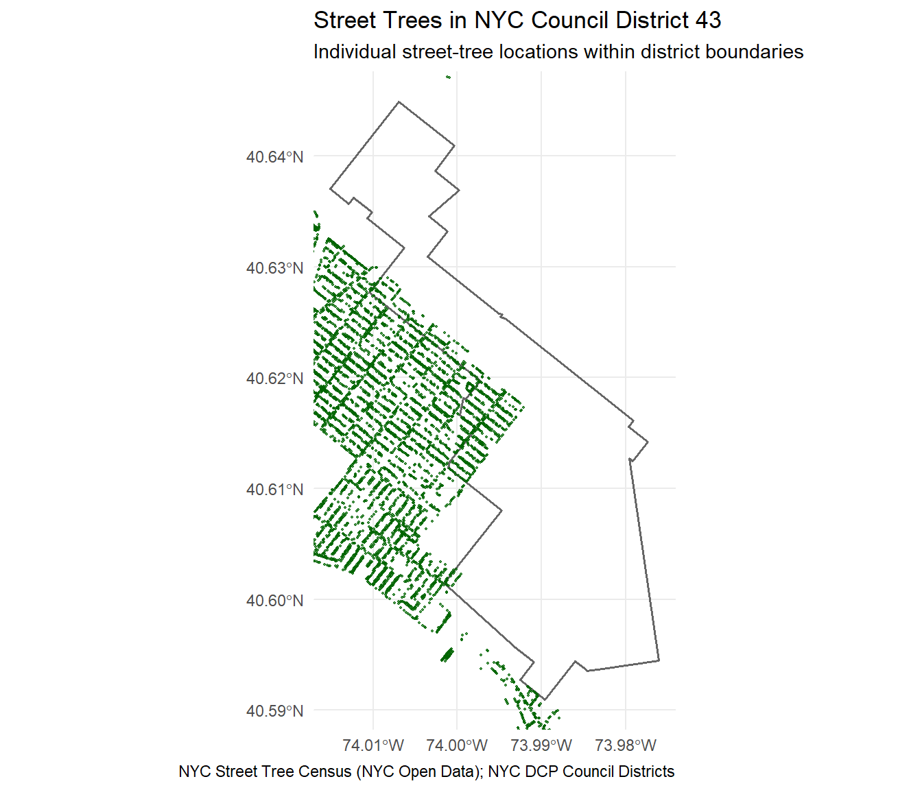
Zoomed-in Map: District 43 Trees
Code
library(sf)library(dplyr)library(ggplot2)focus_dist <-43# District boundarydistrict_43 <- districts |>filter(as.integer(CounDist) == focus_dist)# Extract trees for District 43 using your district columntrees_43 <- trees |>mutate(coun_dist =coalesce(as.integer(council_district),as.integer(cncldist))) |>filter(coun_dist == focus_dist)# PLOT — no colors, no legend, just pointsggplot() +geom_sf(data = district_43, fill =NA, color ="grey40", linewidth =0.7) +geom_sf(data = trees_43, color ="darkgreen", size =0.4, alpha =0.7) +coord_sf(xlim =st_bbox(district_43)[c("xmin", "xmax")],ylim =st_bbox(district_43)[c("ymin", "ymax")],expand =0.02 ) +theme_minimal(base_size =11) +labs(title ="Street Trees in NYC Council District 43",subtitle ="Individual street-tree locations within district boundaries",caption ="NYC Street Tree Census (NYC Open Data); NYC DCP Council Districts" )
Why District 43 (vs. Peers)
Compared to similar districts, District 43 demonstrates both high canopy density and strong tree health, making it an ideal candidate for strategic investment.
Code
peers <-c(focus_dist, peer_dists)compare_df <- dens_by_dist |>select(coun_dist, total_trees, tree_density_km2) |>left_join(dead_by_dist |>select(coun_dist, frac_dead), by ="coun_dist") |>filter(coun_dist %in% peers) |>mutate(total_trees =comma(total_trees),tree_density_km2 =round(tree_density_km2, 1),frac_dead =round(frac_dead *100, 1) # convert to % ) |>rename("trees per km²"= tree_density_km2,"dead trees (%)"= frac_dead )compare_df
  coun_dist total_trees trees per km² dead trees (%)
1        36       9,031         118.5            1.5
2         9       8,391         149.1            2.9
3        43      13,129         173.9            1.6
4        25       7,841         122.8            1.3
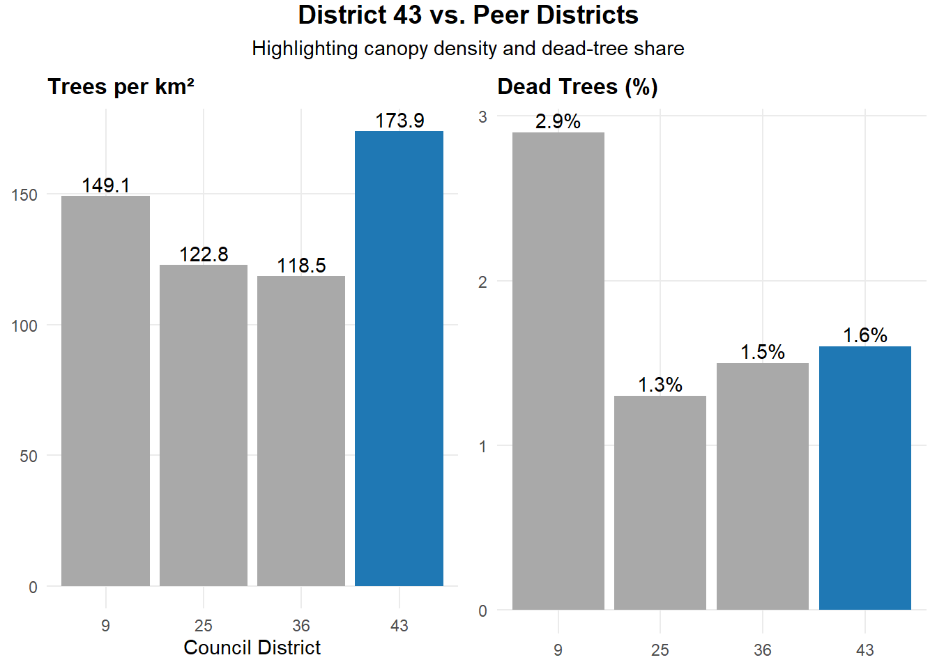
District 43 leads in canopy density yet maintains low mortality, showing strong maintenance but clear opportunities to expand shade coverage in key pedestrian areas. Strategic investment here will build on a solid foundation and benefit a large number of residents.
Non-Map Graphic: Density & Dead Share (D43 vs. Peers)
code
library(cowplot)library(ggplot2)library(dplyr)# Your datacompare_df <- tibble::tribble(~coun_dist, ~dead_share, ~density,43, 1.6, 173.9,9, 2.9, 149.1,25, 1.3, 122.8,36, 1.5, 118.5)compare_df <- compare_df %>%mutate(fill_color =ifelse(coun_dist ==43, "#1f78b4", "#a9a9a9") )# Panel 1 — Trees per km² (NOW FIRST)p_density <-ggplot(compare_df, aes(x =factor(coun_dist),y = density,fill = fill_color)) +geom_col() +geom_text(aes(label = density),vjust =-0.3, size =3.8) +scale_fill_identity() +labs(title ="Trees per km²",x ="Council District",y =NULL ) +theme_minimal(base_size =11) +theme(plot.title =element_text(size =12, face ="bold"),panel.grid.minor =element_blank() )# Panel 2 — Dead Trees % (NOW SECOND)p_dead <-ggplot(compare_df, aes(x =factor(coun_dist),y = dead_share,fill = fill_color)) +geom_col() +geom_text(aes(label =paste0(dead_share, "%")), vjust =-0.3, size =3.8) +scale_fill_identity() +labs(title ="Dead Trees (%)",x =NULL,y =NULL ) +theme_minimal(base_size =11) +theme(plot.title =element_text(size =12, face ="bold"),panel.grid.minor =element_blank() )# Combine side by side — order FLIPPED (p_density first, p_dead second)final_plot <- cowplot::plot_grid( p_density, p_dead,nrow =1,labels =NULL)# Add title + subtitlecowplot::ggdraw() + cowplot::draw_label("District 43 vs. Peer Districts",fontface ="bold", x =0.5, y =0.98, size =14) + cowplot::draw_label("Highlighting canopy density and dead-tree share",x =0.5, y =0.93, size =11) + cowplot::draw_plot(final_plot, x =0, y =0, width =1, height =0.9)
This comparison highlights how District 43’s canopy strength and tree health differ from its peer districts. District 43 has the highest canopy density in the group (173.9 trees per km²), exceeding Districts 9, 25, and 36, which range from 118.5 to 149.1 trees per km². At the same time, District 43 maintains a low dead-tree share of 1.6%, indicating a generally healthy and well-maintained urban forest. Together, these metrics show that District 43 is a strong candidate for strategic canopy expansion, where new plantings can build on a healthy foundation and deliver high environmental value.
Closing & Request
We request $500,000 in funding for the District 43 Urban Canopy Renewal Program to plant new trees, replace aging ones, and improve maintenance across priority corridors. With strong existing canopy density and low mortality, District 43 is well-positioned for cost-effective expansion that will enhance walkability, reduce heat exposure, and support a healthier and more resilient urban environment for residents across Bay Ridge, Dyker Heights, and Bensonhurst.
Conclusion
Overall, this project demonstrates how integrating the NYC Street Tree Census with City Council district boundaries reveals meaningful patterns in canopy density, tree health, and species distribution across the city. By identifying districts with strong coverage as well as those with elevated mortality or limited shade - such as the contrasts observed between District 43 and its peer districts - we can better understand where targeted planting and maintenance efforts will have the greatest environmental and equity impacts. These analyses provide a data-driven foundation for long-term decision-making by the NYC Parks Department, guiding strategic investments in planting, care, and urban canopy resilience citywide.